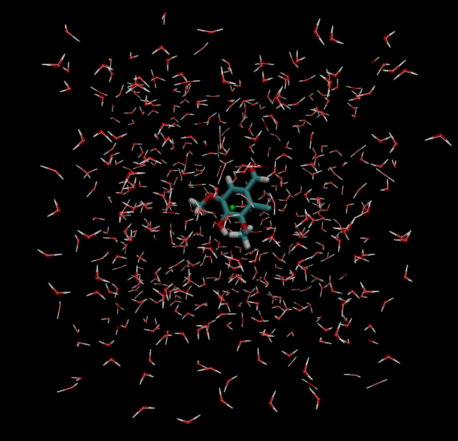
In this tutorial we will calculate the solvation free energy of an organic molecule, 2-chlorosyringaldehyde, in water. 2-chlorosyringaldehyde is a substituted benzene molecule with multiple functional groups:

You could imagine extending this process to other, drug-like small molecules or ligands of interest.
l11.pdb - the structure of the 2-chlorosyringaldehyde molecule ('l11' for short) in PDB format. Download it here.python $PROTOMSHOME/protoms.py -s dualtopology -l l11.pdb --absolute
this sets up a dual topology simulation of the molecule in a box of TIP4P water, perturbing between the full interaction of the molecule with its surroundings and the zero interaction of a dummy atom with its surroundings.
The simulation will run 5 m equilibration steps and 40 m production steps for each of the 16 λ-values. Output will be printed to files every 100 k moves and Hamiltonian replica-exchanges between neighbouring λ-values will be attempted every 200 k moves.
Why dual topology?
For these sorts of absolute free energy calculations (i.e. 'perturbing to nothing'), dual topology simulations will generally provide smoother free energy curves and more precise free energy estimates with smaller errors, particularly at the endpoints of the perturbation. They also have the added advantage that no gas-phase simulations are needed to complete the thermodynamic cycle (see the ProtoMS manual for theory details). Although in theory these calculations can also using a single topology approach, by default protoms.py will suggest you use dual topology. Single topology simulations can be set up using the individual scripts in the tools folder if you prefer.
Why--absolute?
The -s dualtopology argument tells the script to set up a dual topology free energy simulation and the --absolute argument tells the script that no second ligand exists and that the ligand specified by -l should be perturbed to a dummy particle (nothing).
Without the --absolute, the script will expect you to input a second ligand!
Protoms.py will print out a series of information messages if successful, and error messages if there are any problems.
For more detailed information there is also a log file (called protoms_py.log by default), which includes debug messages and defines the values of any command line flags you give to protoms.py, or their default values if you don't set any.
However, the safest way to check is to read over the created files and visualise the created system. You can read more about the files that the setup script creates further down on this page, and you can visualise the system that will be simulated with (for instance) VMD. Note the highlighted dummy atom position in green:
vmd -m l11.pdb l11_dummy.pdb l11_box.pdb
mpirun -np 16 $PROTOMSHOME/protoms3 run_free.cmdThis is most conveniently done on a computer cluster. The calculations take approximately 7 h to complete using the Iridis4 system at the University of Southampton.
out_free folder.
Let's start by evaluating whether the system is well equilibrated. We should first visualise our simulation to check nothing has gone wrong (open out_free/lam-0.000/all.pdb in VMD for example), but we can also use the calc_series.py script to plot the time-dependence of some obvious properties of interest. Type:
python $PROTOMSHOME/tools/calc_series.py -f out_free/lam-0.000/resultsThis will bring up a wizard to look at a choice of various time series of results from the 0.000 λ-window (you can also run
calc_series.py -h to see how to define these choices from the command line).
First of all, let's see how the total energy of the system changes with time. Type total followed by enter twice. This will plot the total energy as a function of simulation snapshot. It should look something like this: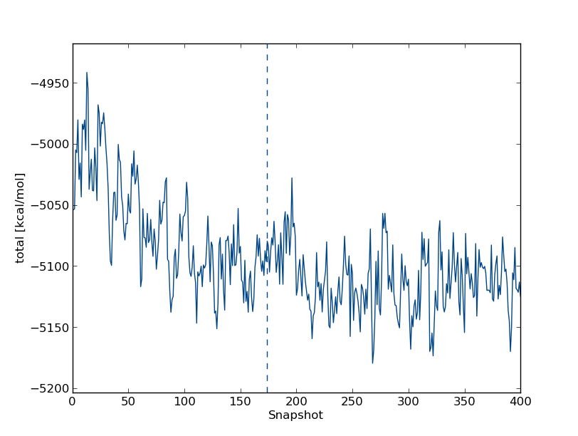
calc_series.py -f out_free/lam-0.000/results again and type:
total
inter/solvent-solvent/sum
inter/l11-solvent/sum
And then choose option 5 for displaying the graphs on the same plot, normalised to the energy of the final snapshot. You should see something like this:
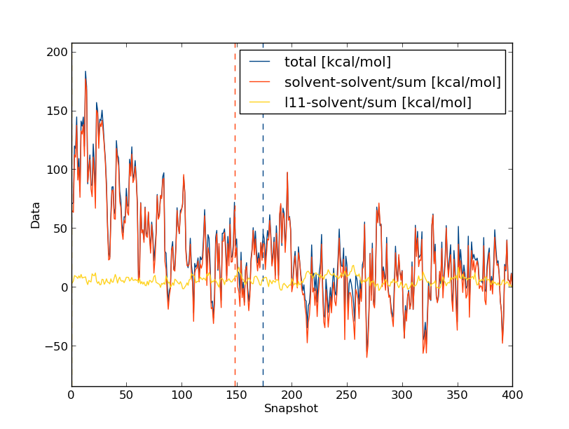
Clearly the change in the total energy is dominated by the solvent-solvent interactions, while the ligand-solvent interactions remain fairly constant throughout. But what effect does this have on the forward & backward free energy differences, and hence the gradients for our TI calculations? Let's take a look, but this time we'll evaluate the trends as running averages and use the command line flags for calc_series.py:
python $PROTOMSHOME/tools/calc_series.py -f out_free/lam-0.000/results --average -s forwfe gradient
This time use option 2 for displaying the graphs as sub-plots, as they have very different scales:
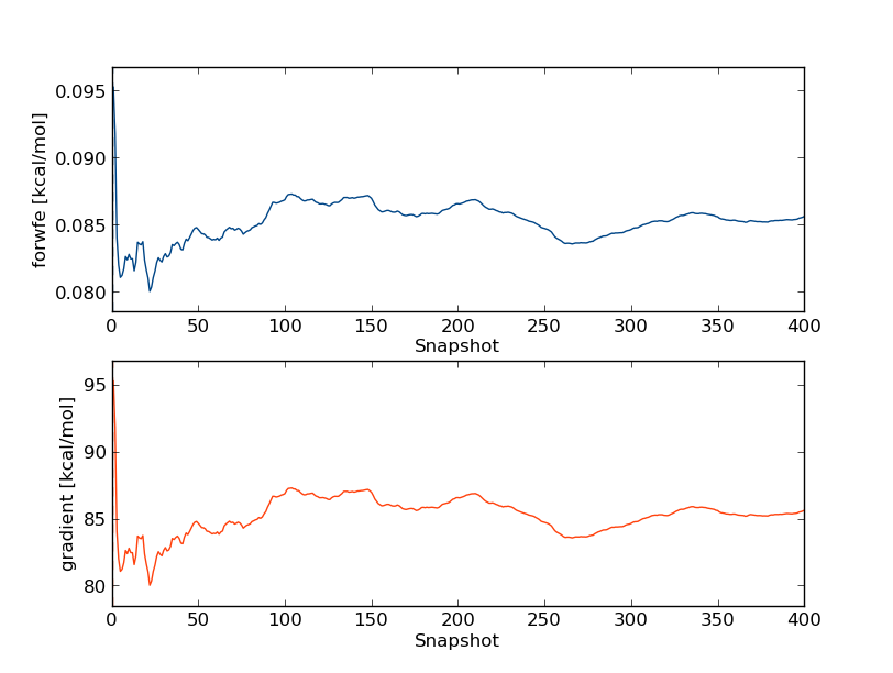
So we can see that the free energy gradients seem fairly constant after around 100 snapshots. Hence we'll discard the first 100 snapshots in our free energy calculations. At this stage we're ready to begin the free energy analysis. We'll do this by Thermodynamic Integration (TI), Bennett's Acceptance Ratio (BAR) and multistate-BAR (MBAR), so we can compare whether the results are sensitive to the choice of estimator. Type:
python $PROTOMSHOME/tools/calc_dg.py -d out_free/ -l 0.25
(The -l flag says we should skip the first 25% of the simulation (100 snapshots) as we decided above). You'll see a table of the dV/dλ gradients followed by the total free energies for the perturbation calculated by TI, BAR and MBAR.
Remember that the free energies given are for the forwards perturbation to nothing. The hydration free energy is the transfer free energy from vacuum to solvent - to opposite of what we've just simulated.
So all we need to do is reverse the sign!
We obtained a value of around -9.3 kcal/mol with TI, -8.4 kcal/mol with BAR and -8.4 kcal/mol with MBAR. The experimental hydration free energy for 2-chlorosyringaldehyde is -7.8 kcal/mol, so although we are fairly close it seems that our computed free energy is slightly dependent on what estimator we choose...but to say for sure we would first have to run more repeats, or try out different simulation conditions.
python $PROTOMSHOME/protoms.py --fullhelp...you can see that there are many different options you can define manually to explore your simulation further! A few examples are given below.
--nequil - this controls the number of equilibration steps--nprod - this controls the number of production stepspython $PROTOMSHOME/protoms.py -s dualtopology -l l11.pdb --absolute --nequil 10E6 --nprod 50E6you will run 10 m equilibration steps and 50 m production steps (instead of the 5 m and 40 m that is default)
python $PROTOMSHOME/tools/calc_replicapath.py -f out_free/lam-*/results -p 1.000 0.800 0.533 0.200 0.000
You'll see a plot something like this created as replica_path.png
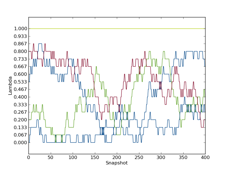
See how the replicas don't traverse the whole of λ-space? Perhaps we could run for longer, or perhaps we could add more windows, and see if the exchange was improved and whether this improved the agreement of our estimators.
The argument that controls the number of λ-values is called --lambdas.
By typing (for instance):
python $PROTOMSHOME/protoms.py -s dualtopology -l l11.pdb --absolute --lambdas 24you will initiate 24 λ-values rather than default 16. You can also give individual λ-values to the argument. For instance:
python $PROTOMSHOME/protoms.py -s dualtopology -l l11.pdb --absolute --lambdas 0.000 0.033 0.067 0.133 0.200 0.267 0.333 0.400 0.467 0.533 0.600 0.667 0.733 0.800 0.867 0.933 0.967 1.000
will add two new λ-values at 0.033 and 0.967 to the 16 created by default.
--repeats or just -r.
by typing for instance:
python $PROTOMSHOME/protoms.py -s dualtopology -l l11.pdb --absolute -r 5you will create 5 input files that will create 5 output folders. But remember, you also need to execute ProtoMS 5 times with the different input files. The output folders will be named e.g.
out1_free,out2_free...
By default, protoms.py solvates systems using the TIP4P water model. Simulations can also be performed with the TIP3P model by using the --watmodel flag:
python $PROTOMSHOME/protoms.py -s dualtopology -l l11.pdb --absolute --watmodel tip3pAlternatively you may wish to solvate the solute using a different pre-equilibrated water box, or create a box of different dimensions. This can be done using the individual solvate script in the tools section.
l11.prepi = the z-matrix and atom types of l11 in Amber format (created by Amber)l11.frcmod = additional parameters not in GAFF (created by Amber)l11.zmat = the z-matrix of l11 used to sample it in the MC simulationl11.tem = the complete template (force field) file for the ligand in ProtoMS formatl11_box.pdb = the box of water solvating l11 in the simulationl11_dummy.pdb = the dummy particle that l11 will be perturbed intol11-dummy.tem = the combined template file for l11 and the dummy, used only in this simulationrun_free.cmd = the ProtoMS input file for the simulation
dualtopology1 1 2 synctrans syncrot
softcore1 solute 1
softcore2 solute 2
softcoreparams coul 1 delta 0.2 deltacoul 2.0 power 6 soft66
lambdare 100000 0.000 0.067 0.133 0.200 0.267 0.333 0.400 0.467 0.533 0.600 0.667 0.733 0.800 0.867 0.933 1.000
protoms.py
l11.pdb contains a directive, telling ProtoMS the name of the solute. The line should read HEADER L11 and can be added using whichever editor you feel most comfortable with. For example:
sed -i "1iHEADER L11" l11.pdb
python $PROTOMSHOME/tools/ambertools.py -f l11.pdb -n L11
This will execute the AmberTools programs antechamber and parmchk, creating the files l11.prepi and l11.frcmod, respectively. If the ligand was charged, we could specify that here using the -c flag.
python $PROTOMSHOME/tools/build_template.py -p l11.prepi -f l11.frcmod -o l11.tem -n L11
This will create the files l11.tem (the ProtoMS template file) and l11.zmat (the ProtoMS z-matrix). It is a good idea to check the latter to see if the script has defined the molecule properly.
python $PROTOMSHOME/tools/solvate.py -b $PROTOMSHOME/data/wbox_tip4p.pdb -s l11.pdb -o l11_box.pdb
As standard this will create a box of mimimum 10 A distance between the solute and the edge of the box. The padding of the box from the solute can be increased using the --padding or -p option.
Likewise a different pre-equilibrated box can be used by specifying the location using the -b flag. The output is written to the file l11_box.pdb.
python $PROTOMSHOME/tools/make_dummy.py -f l11.pdb -o l11_dummy.pdb
This creates l11_dummy.pdb that just contains the new particle.
python $PROTOMSHOME/tools/merge_templates.py -f l11.tem $PROTOMSHOME/data/dummy.tem -o l11-dummy.tem
creating l11-dummy.tem. The template file of the dummy particle is located in $PROTOMSHOME/data/.
Now we have all the files except the ProtoMS input file itself. As you may have noticed, this step-by-step procedure create a few files that protoms.py does not generate, but these often contain logs of the exact procedures performed, so they may be useful to you.
python $PROTOMSHOME/tools/generate_input.py -s dualtopology -l l11.pdb l11_dummy.pdb -t l11-dummy.tem -lw l11_box.pdb --absolute -o run
creating run_free.cmd.