Sampling and equilibration with MUP-I

Sampling the atomistic configurations of biomolecules is what ProtoMS is all about, and represents its most basic functionality. This tutorial will show you how to use Monte Carlo to generate configurations of major urinary protein 1 (MUP-I) complexed with a small molecule (PRZ). In addition, you will learn the importance of equilibration, and how we detect and deal with equilibration in ProtoMS.

Prerequisites

prz.pdb - the PDB structure of the small molecule PRZ
protein.pdb - the PDB structure of the MUP-I

Both the protein and ligand have been protonated, and the protein atoms are in the AMBER naming scheme. The ligand is in its crystallographic pose. There is one cysteine bridge between residues 64 and 157, which have been labelled as CYX. You can read more about setting up structures here.

Simple setup

Setup

All we need to do to set-up a simulation is type

python $PROTOMSHOME/protoms.py -s sampling -p protein.pdb -l prz.pdb

which automatically solvated the system, and using GAFF, generated the forcefield and topolographic information of the ligand. By entering -s sampling , we are telling protoms.py that we wish to sample configurations of the system.

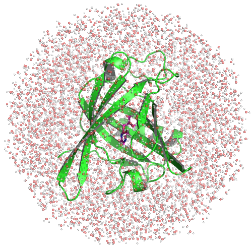
The solvated system should look like this:

The command file run_bnd.cmd was also generated by protoms.py; it summarises everything ProtoMS needs to know about running a simulation. At the bottom of run_bnd.cmd is

dump 100000 results write results
dump 100000 pdb all solvent=all file=all.pdb standard
dump 100000 restart write restart
dump 100000 averages reset
chunk equilibrate 5000000 solvent=774 protein=213 solute=14 volume=0
chunk simulate 40000000 solvent=774 protein=213 solute=14 volume=0

The lines starting with chunk tells ProtoMS what it should be sampling, and whether it should be recording data. The chunk equilibrate 5000000 means that while 5,000,000 sequential system configurations will be generated, data will not be recorded over this period. Following that, chunk simulate 40000000 means that 40,000,000 snap-shots will be generated, and that data will be recorded. This is the only difference between the equilibrate and simulate commands; they both sample the system, but only one can output data. The benefit of using equilibrate is that while the system is relaxing, the data is discarded without taking up any disk space. As chunk simulate comes after chunk equilibrate, the last frame from the equilibration run will be used as the start of the "simulate" chunk.

The lines starting with dump relate to chunk simulate, as they tell ProtoMS the frequency with which it will output the various files while it is simulating; these are the PDBs of the structures, the restart files, as well as the frequency with which cumlative averages (such as the total energy) will be reset.

As mentioned, there is one cysteine bridge in MUP-I. This needs to be constrained as their sampling is not yet properly coded for in ProtoMS. At the top of the protein_pms.pdb file, this is achieved via the following lines:

REMARK chunk fixbackbone 1 63, 65, 156
REMARK chunk fixresidues 1 64, 157

which will also constrain the backbones of the residues immediately adjacent to the cysteine bridge.

Execution

Simply type

$PROTOMSHOME/protoms3 run_bnd.cmd

to simulate the system. This will use one processor and take at least 5 hours to complete.

Analysis

Because of some the time scales involved, this section will analyse a simulation that was twice as long as the one specified in the automatically generated run_bnd.cmd. This was done by changing chunk simulate 40000000 to chunk simulate 80000000 in run_bnd.cmd.

To view a movie of the simulation, you can use VMD:

vmd all.pdb

All there is to see is a lot of atoms wiggling and jiggling. What we're really interested in is how the energies of the system change as the simulation progresses. For instance, type

python $PROTOMSHOME/tools/calc_series.py -f out_bnd/results -s total inter/protein1-solvent/sum inter/solvent-solvent/sum inter/prz-solvent/sum -p sub

which, due to the -s flag, will analyse the total energy (total), solvent-solvent interaction energy (inter/solvent-solvent/sum), protein-solvent interaction energy (inter/protein1-solvent/sum), and the ligand-solvent interaction energy (inter/prz-solvent/sum). The -p sub flag indicates we'd like the plots of energies printed as sub-plots, which, for our 80M move simulation look like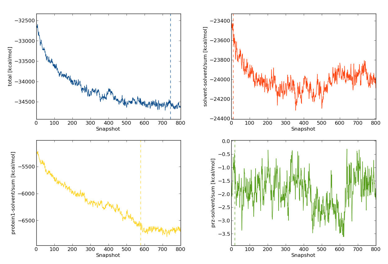

As indicated by the y-axis, the total energy is shown in blue at the top left plot. The intriguing feature of the total energy is that over the course of the simulation, it decreases to what appears to be a constant average value. However, by eye, the total energy only appears to be roughly flat at around the 700th snapshot. As frames were output every 100,000 frames (as specified by the dump commands in run_bnd), 700 snapshots correspond to 70M Monte Carlo moves.

What about equilibration? A necessary, but often insufficient, condition for equilibrium is

"A quantity is said to be at equilibrium if it does not change with time."

Therefore, it appears as if the system composed of water, MUP-I and the ligand PRZ does not reach equilibrium until around 70M moves. Will this energy drift affect free energy calculations? Some insight can be gained by looking at the plots of the other energies we produced, namely the protein-solvent interaction energy (yellow, bottom left). This quantity accounts for much for the decrease in the total energy. The solvent-solvent energy also appears, by eye, to also decrease with time. In contrast, the ligand-solvent energy appears roughly constant over the entirety of the simulation. Before reaching any conclusions about the equilibration of the ligand, let's have a look at the ligand-protein interaction energy. So that you can gain some experience with the interactive mode of calc_series, type

python $PROTOMSHOME/tools/calc_series.py -f results

and, type inter/protein1-prz1/sum and hit the enter key. (Note that you can analyse the Lennard-Jones (lj) and Coulomb (cou) energies separately.) This will produce the ligand-protein interaction energy. In our simulation, we find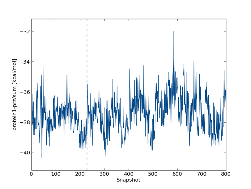

Like the ligand-solvent energy, this quantity appears to vary around a constant value.

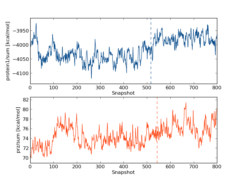
We can also have a look at internal energies of the protein and ligand

python $PROTOMSHOME/tools/calc_series.py -f results -s intra/protein1/sum intra/prz/sum -p sub

These quantities also don't vary much over the course of the simulation. While the total energy ‒ due to protein-solvent energy ‒ does not reach equilibrium for the majority of the simulation, the energies associated with the ligand seem roughly constant. Therefore, if we were to use this data for free energy calculation on the ligand, the lack of drift in these energies would help us trust the numeric answers we get.

The keen eyed among you would have noticed that one every plot is a verticle dashed line, and every time calc_series is called produces output like

Equilibration found at snapshot 543 for prz_sum, value=74.653
	This production part is estimated to contain 20 uncorrelated samples (g=12.472)
	The number of samples is maximized at 485, g=13.850 and the number of uncorrelated samples is 22

This occurs because calc_series is automatically trying to find when a quantity reaches equilibrium. The dashed verticle line and first line of the output are done via a hypothesis test on whether the line is "flat" or not. Data to the left of the dashed line is estimated to be "unequilibrated", and data to the right is estimated to be "equilibrated". By trying to maximise the number of uncorrelated samples, a second estimate of the equilibration point is also produced. While these tools were designed to determine the points of equilibria objectively, they sometimes disagree with human intuition. Have another look at the plots above and see if you agree with the algorithm as to where to equilibration point is.

Files created by the setup script

Simulation specific files

Running make_gcmcbox.py and protoms.py created the following files:

water.pdb = the droplet of solvent water that surrounds the protein and ligand
protein_pms.pdb = the PDB structure of the protein in the ProtoMS naming scheme
prz.tem = the forcefield template file of the ligand PRZ, which contains move information
run_bnd.cmd = the command file that tells ProtoMS what to simulate and how

The following files are also created, although they will not be needed for the equilibration of the protein-ligand-water system:

prx_box.pdb = cubic box of water around the ligand
prz.zmat = the z-matrix of the ligand, used to generate the ligand moves in Monte Carlo
prz.prepi = the AMBER prepi file of the ligand created by antechamber
prz.frcmod = the AMBER frcmod file that is also created by antechamber

The file prz.tem tells ProtoMS the partial charges and Lennard-Jones parameters for each atom in the ligand. It incorporates all the information present in prz.zmat, prz.prepi and prz.frcmod.

Advanced set-up with individual tools

We can be extra careful in the way we set up our system when we use the tools located in the directory $PROTOMSHOME/tools. Here, we will set our simulation up from scratch.

Solvating the system

To solvate the protein with a sphere of water, enter

python $PROTOMSHOME/tools/solvate.py -pr protein.pdb -g droplet -b $PROTOMSHOME/data/wbox_tip4p.pdb -o water.pdb

to make the sphere of solvent in water.pdb. The default radius of the sphere is 30 Å, which is fine in this case. A different radius can be specified by the -r flag.

It is important to consider that solvate.py, which is also called by protoms.py, adds water molecules randomly to the system based on a pre-equilibrated box of water. Water molecules that have been added but sterically clash with the protein or ligand are automatically removed. While this works okay in most situations, MUP-I has a very hydrophobic cavity, meaning that one should think very carefully about if and where one should add waters. With MUP-I, it is prudent to remove all the waters that have been added by solvate.py that are in the binding site. To do so, we will start by creating a box around the ligand that is at least 3 Å away from it

python $PROTOMSHOME/tools/make_gcmcbox.py -s prz.pdb -p 3 -o box.pdb

creating box.pdb, which can be visualsed in a molecular viewer, such as VMD. Any water molecules in water.pdb that are inside box.pdb can be removed

python $PROTOMSHOME/tools/clear_gcmcbox.py -b box.pdb -s water.pdb -o water_clr.pdb

creating water_clr.pdb.

Preparing the ligand and protein

To set-up the ligand from scratch, we use the GAFF forcefield and AMBERTOOLS. These are called via

python $PROTOMSHOME/tools/ambertools.py -f prz.pdb -c 0

where -c 0 tells AMBERTOOLS that PRZ has no net charge. This has created prz.prepi and prz.frcmod. To use these to generate the template file for ProtoMS, type

python  $PROTOMSHOME/tools/build_template.py -n PRZ -p prz.prepi -f prz.frcmod -o prz.tem

which creates prz.tem.

Before proceeding, the protein atom names have to be adapted to the ProtoMS convention. This is done with the command

python $PROTOMSHOME/tools/convertatomnames.py -p protein.pdb -c $PROTOMSHOME/data/atomnamesmap.dat

The files above need to be reference by the ProtoMS command file, created using

python $PROTOMSHOME/tools/generate_input.py -p protein_pms.pdb -l prz.pdb -t prz.tem -pw water_clr.pdb -s sampling -o run_bnd.cmd --outfolder out_bnd --nprod 80000000 --nequil 5000000

creating run_bnd.cmd. Note that here we specify how long we want our equilibration and simulation time to be. If you recall, the data from the equilibration moves are not recorded. In the above, we specified that we want 5M moves of equilibration, and 80M moves for the production step. Given that it took roughly 70M moves for the total energy to equilibrate, if that were our quantity of interest, a much longer equilibration run would be necessary.

Finally, because there is a cysteine bridge in MUP-I, we need to add

REMARK chunk fixbackbone 1 63, 65, 156
REMARK chunk fixresidues 1 64, 157

to the REMARK section of the protein_pms.pdb file.