Estimating the binding affinity of water molecules

In this tutorial, you will estimate the binding affinity of three conserved water molecules in the binding cavity of the N-terminal domain of HSP90 with a small fragment bound¹. To achieve this we will use the JAWS² technique.

To come back to the tutorial index, click here.

Prerequisites

fragment.pdb - the structure of the small fragment molecule in PDB format
protein.pdb - the structure of the N-terminal domain of HSP90 in PDB format
jaws2_waters.pdb - The structure of the waters which binding affinity we will determine

Both the fragment and protein have been prepared for use with ProtoMS. For instance, they have been protonated. You can read more about setting up structures here.

The file jaws2_waters.pdb needs to be in the appropriate format. If you wish to run JAWS stage 2 from the output clusters from a JAWS stage 1 calculation, you do not need to make any changes to the format. In the appropriate section below, there is an explanation on how to change the format of your waters to the appropriate format for this calculations. For the purpose of this tutorial, your file jaws2_waters.pdb is already in the correct format.

Simple setup

Setup

The simplest way to setup the simulation is by typing the following

python $PROTOMSHOME/protoms.py -s jaws2 -l fragment.pdb  -p protein.pdb --gcmcwater jaws2_waters.pdb --jawsbias 8 10 12 14

this sets up one JAWS stage 2 simulation, to estimate the binding affinty of the waters given in jaws2-waters.pdb, assuming the an on/off ratio close to one will be obtained with jawsbias of 8 to 14. This command will produce one ProtoMS input file per water molecule. Each of the simulations will run 5 m equilibration steps and 40 m production steps. Output will be printed to files every 100,000 moves.

The -s jaws2 argument tells the script to setup a JAWS stage 2 simulation. The -p and -l arguments specifies the protein and the ligand, respectively. After the --gcmcwater flag, the pdb file with the waters whose binding affinities we want to calculate should be specified. The --jawsbias flag corresponds to a JAWS stage 2 specific parameter. It can be understood as a force applied to the water molecules, increasing their likelihood of being off as we increase the value of the bias. We wish to apply a jawsbias such that the ratio of simulation steps during which the considered water was at high theta values (on) with respect to the time spent at low thetas (off) is as close to 1 as possible. More on jawsbias can be read in the ProtoMS manual.

You can read more about the files that the setup script creates further down on this page.

Execution

To run the simulation for one of the water molecules you need to execute

mpirun -np 4 $PROTOMSHOME/protoms3 run_jaws2-w1_jaws.cmd > run_w1.out

Where the number after -np stands for the number of cores which the simulation will use, and should be set to as the same as the number of jawsbias values. The calculations may take up to 10 hours to complete.

Analysis

When the simulations are finished you need to analyse the simulations to produce an estimate for the binding affinity of each of your waters. The analysis will be independent for each of the water molecules.

In the out folder produced (out_jaws2-w1), different directories for each jawsbias value will be placed, and a results can be found in each of these. Within this results file, information on the proportion of moves spent at high and low theta values is printed at the end of each information dump (starting with the line RESULTS FILE). All of the simulation moves are taken into acount in the last information dump, so we only really need to look at the last lines of the file. These last lines will look similar to this:

####################################################
JAWS-2 moves with theta above 0.95 - centre position
####################################################
 HIGH     2197270   59.785316428542785        31.516200149459788        27.603962363437134
####################################################
JAWS-2 moves with theta below 0.05 - centre position
####################################################
 LOW     2591119   59.587933149584636        30.699611271801380        27.297105422389237

Look for the jawsbias for which the ratio between the HIGH and the LOW moves is closer to one. Now an estimation on whether the ratio is close enough to one has to be made. As a guide, a ratio between 0.8 and 1.2 is probably acceptable. If such ratio is not found in any of your simulations, you are advised to re-run this simulations with a more appropriate range of jawsbias values.

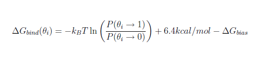
When the desired jawsbias output has been chosen, the binding free energy of the water can be estimated following the formula shown below:

where P(θ→1)/P(θ→0) is approximated from the proportion of moves spent at high theta values with respect to the moves spent at low theta values.

This same analysis procedure should be followed for each of the water molecules for which binding affinity is to be calculated.

As an example, if the results file shown above is found with an applied jawsbias of +10kcal/mol, the consequent binding free energy of the water molecule is estimated to be -3.4kcal/mol. This was the case of one run for the first of the waters in the jaws2_waters.pdb file provided. Please bear in mind this method is inherently noisy.

Exploring more options

Changing the format of the water pdb file

For the JAWS stage 2 calculation to work, the pdb file containing the waters for which binding affinity is to be calculated needs to be in a specific format. An example of this format is displayed below:

HEADER WA1
ATOM      1 O00  WA1  2137      61.033  30.884  27.763        
ATOM      2 H01  WA1  2137      60.475  31.645  27.603        
ATOM      3 H02  WA1  2137      60.548  30.084  27.561        
ATOM      4 M03  WA1  2137      60.891  30.879  27.714   
TER     
ATOM      1 O00  WA1  2139      60.771  34.710  23.191        
ATOM      2 H01  WA1  2139      61.285  34.865  23.983        
ATOM      3 H02  WA1  2139      60.076  34.079  23.379        
ATOM      4 M03  WA1  2139      60.746  34.645  23.324   
TER     
ATOM      1 O00  WA1  2068      62.808  32.279  29.365        
ATOM      2 H01  WA1  2068      62.660  32.932  30.049        
ATOM      3 H02  WA1  2068      62.376  31.460  29.608        
ATOM      4 M03  WA1  2068      62.729  32.256  29.491

If the water pdb file was obtained by any other method which is not the result of a JAWS stage 1 calculation, it is likely that the format will not correspond to that shown above. However, the transformation to the desired format should be as easy as typing:

python $PROTOMSHOME/tools/convertwater.py -p waters_in.pdb -o jaws2_waters.pdb -n WA1

Where the name of the pdb files containing the waters in the original format is introduced after the flag -p and the name of the ouput pdb file after -o . This script will transform your waters to TIP4P-like waters, but with the necessary residue and atom names. Please check the output generated by this script. If no satisfactory changes were made, try changing the residue names if your original pdb to 'SOL' or 'HOH' and then type the command given above.

Once the waters are in the correct format, please remember to include the header in the first line, as displayed in the example above.

Running independent simulations for each `jawsbias`

It is also possible to set up the input files and run ProtoMS for one individual jawsbias. The whole procedure is basically identical. The execution command will differ:

$PROTOMSHOME/protoms3 run_jaws2-w1_jaws.cmd

and in the generated out folder out_jaws2-w1 there will be no folders for each bias.

Running longer simulations

There are two arguments that you can invoke to run a longer simulation

--nequil - this controls the number of equilibration steps
--nprod - this controls the number of production steps

by typing for instance

python $PROTOMSHOME/protoms.py -s jaws2 -p protein.pdb -l fragment.pdb --gcmcwater jaws2_waters.pdb --jawsbias 8 10 12 14 --nequil 10E6 --nprod 50E6

you will run 10 m equilibration steps and 50 m production steps (instead of the 5 m and 40 m that is default)

Running independent repeats

Usually it is wise to run several independent repeats of your calculation to check for convergence. The argument that controls the number of independent repeats is called --repeats or just -r.

by typing for instance

python $PROTOMSHOME/protoms.py -s jaws2 -p protein.pdb -l fragment.pdb --gcmcwater jaws2_waters.pdb --jawsbias 8 10 12 14 -r 5

you will create 5 input files for the JAWS calculation. Therefore, you also need to execute ProtoMS 5 times per water molecule with the different input files. The output will be in 5 different folders per water molecule, e.g. out1_jaws2-w1 and out2_jaws2-w1.

Files created by the setup script

Files describing the fragment

fragment.prepi = the z-matrix and atom types of the fragment in Amber format
fragment.frcmod = additional parameters not in GAFF
fragment.zmat = the z-matrix of the fragment used to sample it in the MC simulation
fragment.tem = the complete template (force field) file for the fragment in ProtoMS format

You can read more about the setup of ligands here.

Files describing the protein

protein_scoop.pdb = the truncated protein structure

You can read more about the setup of proteins here.

Simulation specific files

A few of the files generated are related the the jaws2 waters:

jaws2_wat1.pdb = the pdb of the first of the jaws2 water molecules, in isolation
jaws2_wat2.pdb = the pdb of the second of the jaws2 water molecules, in isolation
jaws2_not1.pdb = the pdb of all the jaws2 waters except for the first. It is used as part of the simulation solvent when jaws2 is run for the first water
jaws2_not2.pdb = the pdb of all the jaws2 waters except for the second. It is used as part of the simulation solvent when jaws2 is run for the second water

whilst others are general simulation files:

water.pdb = the cap of water solvating the protein-ligand system
run_jaws2-w1_jaws.cmd = the ProtoMS input file for the JAWS stage 2 simulation on the first water of those provided
run_jaws2-w2_jaws.cmd = the ProtoMS input file for the JAWS stage 2 simulation on the second water of those provided

You can read more about the input files in the ProtoMS manual. However, some sections of it are worth mentioning here:

jaws2 1
multijaws2 8.000 10.000 12.000 14.000

In the lines seen above, the jaws2 line indicates the initial value of θ for the jaws2 water being considered. The multijaws2 line sets the different values of jawsbias at which the simulation will be run. When only one jawsbias has been specified, the equivalent line in the input file starts with jbias instead.

originx 59.533
originy 29.384
originz 26.263
x 3.0
y 3.0
z 3.0

These lines include the dimensions of the JAWS-box, to which the jaws2-water is constrained. The originx, originy, originz, x, y, z parameters indicate the origin and length of the JAWS-box in each spatial coordinate.

Setting up the simulation with individual tools

In this advanced section we will go through the setup of the simulations step-by-step using individual setup scripts rather than protoms.py. This is relevant in cases where you are interested in specifying certain parameters which are pre-determined by protoms.py.

Setting up the ligand

We will start setting up the ligand from the initial fragment.pdb.

First we need to make sure that the very first line of the fragment.pdb contains a directive, telling ProtoMS the name of the solute. The line should read HEADER XDK, where xdk is the residue name in the fragment, and can be added by typing

sed -i "1iHEADER XDK" fragment.pdb

Thereafter, we will create the force field for the fragment using AmberTools. The force field will be GAFF with AM1-BCC charge. Type

python $PROTOMSHOME/tools/ambertools.py -f fragment.pdb -n XDK

and this will execute the AmberTools programs antechamber and parmchk, creating the files fragment.prepi and fragment.frcmod, respectively.

These files are in Amber format and in order to use them in ProtoMS we need to reformat them into a ProtoMS template file. This file will also contain a z-matrix that describes how the ligand will be sampled during the simulation. To do this, you can type

python $PROTOMSHOME/tools/build_template.py -p fragment.prepi -f fragment.frcmod -o fragment.tem -n XDK

this will creates the files fragment.tem containing the ProtoMS template file and fragment.zmat. It is a good idea to check this files to see if the script has defined the molecule properly.

Now we have setup the fragment, but there is another "ligand" that we have not mentioned: the water molecules used for the JAWS calculation. These are considered by protoms as "grand canonical solutes", and will be generated later, but it is important to mention here that they will, as well, need a template. However, there is no need to generate this template, since it contains some particularities and it can be found in $PROTOMSHOME/data/gcmc_wat.tem.

Setting up the protein

First, we will change the name of atom and residue names in the protein PDB-file such that they agree with the ProtoMS naming convention. Type

python $PROTOMSHOME/tools/convertatomnames.py -p protein.pdb -o protein_pms.pdb -s amber -c $PROTOMSHOME/data/atomnamesmap.dat

The converted structure will be in protein_pms.pdb. This execution assumes that the Amber naming convention is used in protein.pdb.

If we have crystallographic waters in the protein structure (which we do not in this example), we need to convert them to the water model we will be using in the simulation (TIP4P). This can be done by

python $PROTOMSHOME/tools/convertwater.py -p protein_pms.pdb -o protein_pms_t4p.pdb

creating protein_pms_t4p.pdb.

Next step is to truncate the protein, creating a scoop. This will enable us to solvate the protein in a droplet and thereby reduce the number of simulated particles. The command is

python $PROTOMSHOME/tools/scoop.py -p protein_pms_t4p.pdb -l fragment.pdb -o protein_scoop.pdb

The protein scoop is centred on the fragment molecule and all residues further than 20 A are cut away. The scoop is written to protein_scoop.pdb

Setting up the solvation and JAWS waters

First we will create a droplet of TIP4P water molecules around both ligand and protein. To do this, type:

python $PROTOMSHOME/tools/solvate.py -b $PROTOMSHOME/data/wbox_tip4p.pdb -s fragment.pdb -pr protein_scoop.pdb -o water.pdb -g droplet

this will create a droplet with 30 A radius centred on the fragment molecule. The droplet is written to water.pdb

The solvate.py script adds the crystallographic waters from the scoop to the droplet. Therefore, we need to remove them from the scoop PDB-file, to avoid duplicates.

sed -i -e "/T4P/d" -e "/TER/d" protein_scoop.pdb

Next we need to split the jaws2 waters into pdbs with individual waters and with all waters except one. It can be done by running:

python $PROTOMSHOME/tools/split_jawswater.py -w jaws2_waters.pdb -o jaws2_ --jaws2box

with this command, the files jaws2_watX.pdb and jaws2_notX.pdb will be generated (where X is a number that goes from 1 to the number of jaws2 waters). They should contain all required information on the jaws2-waters.

The last step in this section consists of clearing the water molecules from the solvation droplet which overlap with the any of the jaws2-box. Do this by typing:

python $PROTOMSHOME/tools/clear_gcmcbox.py -b jaws2_wat1.pdb -s water.pdb -o water.pdb

This command should be run again for each of the pdb files of the individual water molecules.

Now we have all the files need to run the simulation. As you noticed, there is some difference in the files produced with this step-by-step procedure and those created with protoms.py.

Making ProtoMS input files

To make the input files for ProtoMS type

python $PROTOMSHOME/tools/generate_input.py -s jaws2 -p protein_scoop.pdb -l fragment.pdb -t fragment.tem -pw "water.pdb jaws2_not1.pdb" -o run_jaws2-w1 --jawsbias 8 10 12 14 --gcmcwater jaws2_wat1.pdb  --outfolder out_jaws2-w1

creating run_jaws2-w1_jaws.cmd. Remember to repeat this command for each of the jaws2 water molecules.

References

1. Murray et.al. J. Med. Chem., 2010, 53(16), pp 5942-5955

2. Michel et.al. J. Phys. Chem. B, 2009, 113(40), pp 13337-13346