Binding free energy of benzene to T4 lysozyme

In this tutorial, you will setup, run and analyse the calculation of the binding free energy of benzene to the protein T4 lysozyne.

To come back to the tutorial index, click here.

Prerequisites

benzene.pdb - the structure of the benzene molecule in PDB format
protein.pdb - the structure of the T4 lysozyme in PDB format

Both the benzene and protein would need to be prepared before they are used with ProtoMS. For simplicity, tutorial input files have been prepared in advance, but it still is good practice to check. For instance, you must make sure that they are correctly protonated. You can read more about setting up structures here.

Simple setup

Setup

The simplest way to setup the simulation is by typing the following

python $PROTOMSHOME/protoms.py -s dualtopology -p protein.pdb -l benzene.pdb --absolute

this sets up one simulation for the bound leg and one for the free leg of the double-decoupling free energy cycle.

The simulations will run 5 m equilibration steps and 50 m production steps for each of the 16 λ-values. Output will be printed to files every 100 k moves and Hamiltonian replica-exchanges between neighbouring λ-values will be attempted every 100 k moves.

the -s dualtopology argument tells the script to setup a dual topology free energy simulation and the --absolute argument tells the script that no second ligand exists and that the given ligand should be perturbed to a dummy particle (nothing). The -p and -l arguments specifies the protein and the ligand, respectively.

You can read more about the files that the setup script creates further down on this page.

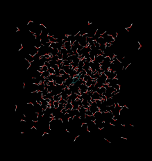
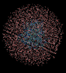
You can visualise the systems that will be simulated with (for instance) VMD:

vmd -m benzene.pdb benzene_dummy.pdb benzene_box.pdb
vmd -m benzene.pdb benzene_dummy.pdb protein_scoop.pdb water.pdb

Execution

To run the bound and free legs of the simulation you need to execute

mpirun -np 16 $PROTOMSHOME/protoms3 run_bnd.cmd
mpirun -np 16 $PROTOMSHOME/protoms3 run_free.cmd

This is most conveniently done on a computer cluster. The calculations will take up to 24 h to complete.

Analysis

When the simulations are finished you need to analyse the simulation and extract the free energy of the bound and free legs. We will start with looking at some energy series to investigate whether the simulations are converged. Type

python $PROTOMSHOME/tools/calc_series.py -f out_free/lam-0.000/results

to look at time series for the free leg at λ=0.0. In the wizard that appears you can type total followed by enter twice. This will plot the total energy as a function of simulation snapshot. It should look something like this:

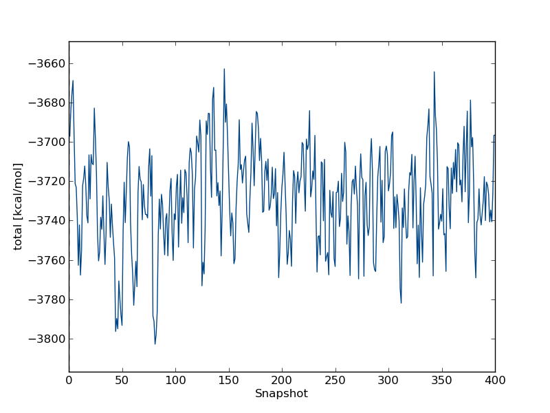
the program will also give you some indication of the equilibration of this time series. In this case, you should see equilibration fairly early in the simulation. Thus, we have to discard very little of the simulation when we compute the free energy.

Next, we will analyse how effective the λ replica exchange was. Type

grep "lambda swaps" out_free/lam-0.000/info

and this will give you the overall acceptance ratio of the λ swaps. It should be around 60% for this perturbation, indicating that the overall effectiveness is acceptable. Next, we will look at individual replicas and see how they exchange λ-value throughout the simulation. This can be done with

python $PROTOMSHOME/tools/calc_replicapath.py -f out_free/lam-*/results -p 0.0 0.2 0.8 1.0 -o replica_path_free.png

to plot the path of the first few λ-values. It should look something like this.

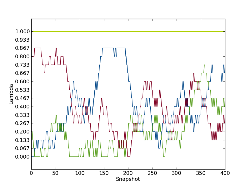
as is clear, these the replicas was not able to traverse the full λ-space within the simulation time. Also the replica starting with λ=1.0, did not exchange a single time throughout the simulation. Hence, the replica exchange was not fully efficient.

Now, we will estimate the free energy. We will do this both with thermodynamic integration, Bennett's acceptance ratio (BAR) and multistate BAR (MBAR). To do this you can type

python $PROTOMSHOME/tools/calc_dg.py -d out_free/ -l 0.025

A typical result is between 0 and 1 kcal/mol. The experimental hydration free energy of benzene is -0.9 kcal/mol, thus this free-leg should be fairly accurate. Notice that only 10 snapshots (2.5% of the simulation) are removed from the 400 snapshots when calculating the free energy, because the analysis with calc_series.py indicated that the simulation was equilibrated very much from the start.

It is important to study the gradient of the TI calculation. It should be smooth in order for the TI to work properly. For the free leg it should look something like this

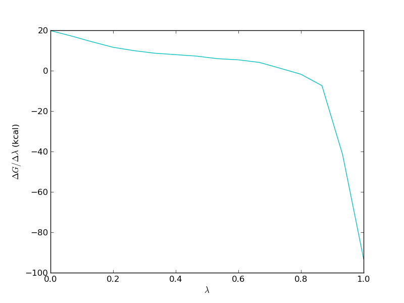
Now, we need to repeat the analysis for the bound leg. When you plot the evolution of the total energy using calc_series.py you will often find that it takes a very long time for the total energy to converge. This is because in the bound simulation, the total energy is dominated by solvent-solvent and protein-solvent interactions that have very little effect on the free energy of binding. Thus we should not look at the total energy when investigating convergence, rather we should look at the interaction between the ligand and either protein or solvent.
Type

python $PROTOMSHOME/tools/calc_series.py -f out_bnd/lam-0.000/results

and when you're prompted for the series to analyze, type the following series

total
inter/solvent-solvent/sum
inter/protein1-solvent/sum
inter/bnz-solvent/sum
inter/protein1-bnz/sum

and when asked for the type of plot, simply select option 5. The plot should look something like this.

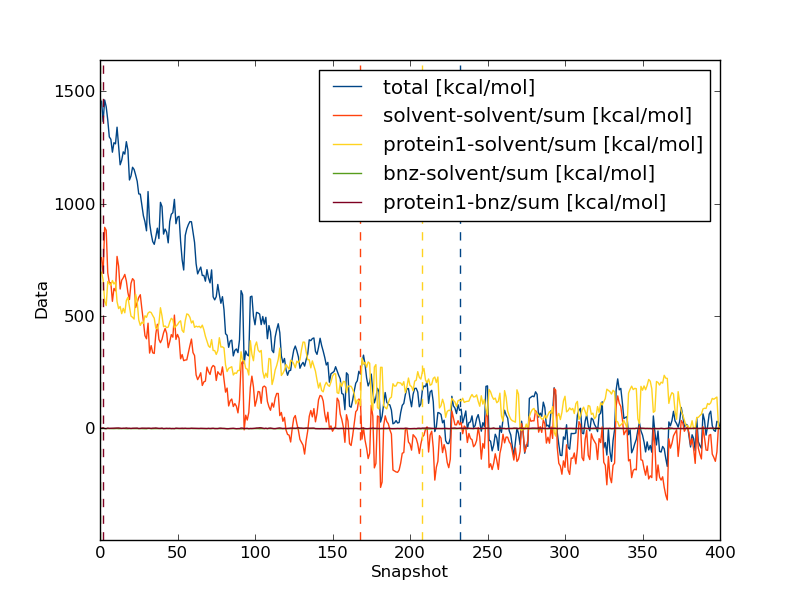
You will notice that the interaction energy between the ligand and its surrounding equilibrates very quickly. The computed free energy should be between 9.0 and 10.0 kcal/mol (depending on estimator and equilibration removed).

As we have decoupled the ligand whilst using a restraint there are two additional correction terms that must be calculated. These are the free energy to introduce the restraint whilst the ligand is in the protein (ΔG_rest1) and the free energy to release the restraint in the gas phase (ΔG_rest2). As the second term is for the gas phase it has a simple analytical form that also incorporates a standard state correction. This is evaluated as the following: ΔG_rest2 = RT ln ( V_sim / V₀ ), where RT is the gas constant multiplied by the absolute temperature and V₀=1660 A³. The simulation volume of benzene V_sim can be estimated from (2πRT / k)^3/2 where k is the harmonic spring constant. With a spring constant of 2 kcal / mol. ΔG_rest2 should evaluate to -3.84 kcal/mol. (Note that ProtoMS defines the harmonic restraint using k, rather than 0.5 k, the above formula for the simulation volume is correct for a restraint with 0.5 k).

Unfortunately, the bound phase restraint term, ΔG_rest1, has no simple solution and must be calculated from an additional simulation. The file run_bnd_rstr.cmd was also created by the setup tools. It performs a replica exchange free simulation for the bound phase system with and without the restraint. This can be executed with:

mpirun -np 2 $PROTOMSHOME/protoms3 run_bnd_rstr.cmd

and will create the output folder out_bnd_rstr. The free energy to introduce the restraint is then calculated similarly to before:

python $PROTOMSHOME/tools/calc_dg.py -d out_bnd_rstr/ -l 0.375 -e bar

where the amount of skipped data is chosen as above. Only the free energy difference calculated using BAR is requested as the trapezium rule used to evaluate TI cannot be considered accurate with only 2 λ values as here. This should evaluate to ~1 kcal/mol.

The standard binding free energy of benzene can then be estimated from:

ΔG_bind = ΔG_free – ΔG_bound – ΔG_rest1 – ΔG_rest2

and it should evaluate to between -5.4 and -5.9 kcal/mol. The experimental value is -5.2 kcal/mol, so the computational prediction is pretty good!

Exploring more options

By running protoms.py as above, you accept the standard number of λ-values, simulation length etc. The values of these parameters were chosen from experience and should work for most systems. However, there are situations when you may want to do something else. Here, we will go through some of the many available options. To know about other options you have to read the manuals for the tools or the overall MC program. You might also have to set up your system by executing the individual tools separately.

Running longer simulations

There are two arguments that you can invoke to run a longer simulation

--nequil - this controls the number of equilibration steps
--nprod - this controls the number of production steps

by typing for instance

python $PROTOMSHOME/protoms.py -s dualtopology -p protein.pdb -l benzene.pdb --absolute --nequil 10E6 --nprod 50E6

you will run 10 m equiliration steps and 50 m production steps (instead of the 5 m and 40 m that is default)

Running with more λ-values

The argument that controls the number of λ-values is called --lambdas.

by typing for instance

python $PROTOMSHOME/protoms.py -s dualtopology -p protein.pdb -l benzene.pdb --absolute --lambdas 24

you will initiate 24 λ-values rather than default 16. You can also give individual λ-values to the argument. For instance

python $PROTOMSHOME/protoms.py -s dualtopology -p protein.pdb -l benzene.pdb --absolute --lambdas 0.000 0.033 0.067 0.133 0.200 0.267 0.333 0.400 0.467 0.533 0.600 0.667 0.733 0.800 0.867 0.933 0.967 1.000

will add two new λ-values at 0.033 and 0.967 to the 16 created by default.

Running independent repeats

Usually it is wise to run several independent repeats of your calculation to check for convergence and to obtain a good estimate of the statistical uncertainty. The argument that controls the number of independent repeats is called --repeats or just -r.

by typing for instance

python $PROTOMSHOME/protoms.py -s dualtopology -p protein.pdb -l benzene.pdb --absolute -r 5

you will create 5 input files for the bound leg and 5 input files for the free leg. Therefore, you also need to execute ProtoMS 10 times with the different input files. The output will be in 10 different folders, e.g. out1_bnd and out2_bnd.

Running with temperature replica-exchange

To improve sampling, one could add temperature ladders to the simulation and perform replica-exchange swaps between neighboring values of temperatures. To add eight additional temperatures to λ-values 0 and 1.0, add the following lines to the command file(s) (files ending in .cmd).

temperaturere 1E5 25.0 27.0 30.0 34.0 39.0 45.0 52.0 60.0 69.0
temperatureladder lambda 0.00 1.00 
lambdaladder temperature 25.0

The last line indicates that the lambda replica exchange will occur at 25 degrees Celsius. It should be noted that the selection of temperatures is a non-trivial task and it is likely to be system dependent. The above lines should therefore be regarded as a suggestion. ProtoMS then needs to be executed with additional nodes, for instance

mpirun -np 32 $PROTOMSHOME/protoms3 run_bnd.cmd

Optimizing the harmonic restraint

The harmonic restraint added by protoms.py is by default 1 kcal/mol/A². It can sometimes be necessary to optimize it so that the free energy is not affected by the magnitude of the restraint. This can be done by running a short unrestrained simulation and estimate the force constant from the root mean square deviation by applying the equipartition theorem.

To setup the short unrestrained simulation, first make a separate folder for the simulation. Then you can type

python $PROTOMSHOME/protoms.py -s sampling -p protein.pdb -l benzene.pdb --nprod 500E3 --nequil 0 --dumpfreq 1E3

$PROTOMSHOME/protoms3 run_bnd.cmd

this 50 k simulation should only take about five minutes to execute. The simulation output can be found in out_bnd.

To calculate the RMSD and estimate an appropriate force constant, type

python $PROTOMSHOME/tools/calc_rmsd.py -i benzene.pdb -f out_bnd/all.pdb -l BNZ -a C4

where BNZ is the residue name of the ligand, and C4 is the atom the restraint is applied to. The output should be something like this.

The RMSD of the atom c4 is 0.898 A

This corresponds to a spring constant of 2.205 kcal/mol/A2
(to use this as an harmonic restraint in ProtoMS, specify 1.102)

and we can see that the default force constant is appropriate. The force constant is estimated from k = 3 RT / <RMSD²>, where R and T are the gas constant and the absolute temperature, respectively. Notice that in the ProtoMS input you specify 1/2k rather than k.

Files created by the setup script

Files describing benzene

benzene.prepi = the z-matrix and atom types of benzene in Amber format
benzene.frcmod = additional parameters not in GAFF
benzene.zmat = the z-matrix of benzene used to sample it in the MC simulation
benzene.tem = the complete template (force field) file for the ligand in ProtoMS format

You can read more about the setup of ligands here.

Files describing the protein

protein_scoop.pdb = the truncated protein structure

You can read more about the setup of proteins here.

Simulation specific files

benzene_box.pdb = the box of water solvating benzene in the free leg simulation
water.pdb = the cap of water solvating the protein-ligand system in the bound leg simulation
benzene_dummy.pdb = the dummy particle that benzene will be perturbed into
bnz-dummy.tem = the combined template file for benzene and the dummy, used only in this simulation
run_bnd.cmd = the ProtoMS input file for the bound-leg simulation
run_free.cmd = the ProtoMS input file for the free-leg simulation

You can read more about the input files in the ProtoMS manual. However, some sections of it are worth mentioning here

dualtopology1 1 2 synctrans syncrot
softcore1 solute 1
softcore2 solute 2
softcoreparams coul 1 delta 0.2 deltacoul 2.0 power 6 soft66

this section, which exists in both input files, sets up the dual topology simulation with appropriate soft-core parameters. It could be worth trying to optimize the soft-core parameters if your simulation is not performing well.

lambdare 100000 0.000 0.067 0.133 0.200 0.267 0.333 0.400 0.467 0.533 0.600 0.667 0.733 0.800 0.867 0.933 1.000

this section, which exists in both input files, sets up the λ-replica exchange. You can add more λ-values manually if there are regions where the simulation is not performing well.

chunk id add 1 solute 1 C4 BNZ
chunk restraint add 1 cartesian harmonic 27.837 6.921 3.569 1
chunk id add 2 solute 2 C1 DDD
chunk restraint add 2 cartesian harmonic 26.911 6.126 4.178 1

this section, which is unique for the bound-leg simulation, restrains the benzene and the dummy particle to the binding site with harmonic restraints. It could be worth trying to optimize the weight of the restraint or try another type of restraint if your simulation is not performing well. This is discussed here.

Setting up the simulation with individual tools

In this advanced section we will go through the setup of the simulations step-by-step using individual setup scripts rather than protoms.py

Setting up the free leg

We will start setting up the free-leg simulation. However, it should be noted that some of the files created in this section will also be used in the bound-leg simulation.

First we need to make sure that the very first line of the benzene.pdb contains a directive, telling ProtoMS the name of the solute. The line should read HEADER BNZ and can be added by typing

sed -i "1iHEADER BNZ" benzene.pdb

Thereafter, we will create the force field for the benzene molecule using AmberTools. The force field will be GAFF with AM1-BCC charge. Type

python $PROTOMSHOME/tools/ambertools.py -f benzene.pdb -n BNZ

and this will execute the AmberTools programs antechamber and parmchk, creating the files benzene.prepi and benzene.frcmod, respectively.

These files are in Amber format and in order to use them in ProtoMS we need to reformat them into a ProtoMS template file. This file will also contain a z-matrix that describes how benzene will be sampled during the simulation. To do this, you can type

python $PROTOMSHOME/tools/build_template.py -p benzene.prepi -f benzene.frcmod -o benzene.tem -n BNZ

this will creates the files benzene.tem containing the ProtoMS template file and benzene.zmat. It is a good idea to check these files to see if the script has defined the molecule properly.

The next thing we will do is to solvate the benzene molecule in a box of TIP4P water molecules. Type

python $PROTOMSHOME/tools/solvate.py -b $PROTOMSHOME/data/wbox_tip4p.pdb -s benzene.pdb -o benzene_box.pdb

this will solvate benzene using standard settings, i.e. it will be 10 A between the solute and the edge of the box. A pre-equilibrated box of TIP4P water molecules located in $PROTOMSHOME/data/ is used. The box is written to the file benzene_box.pdb.

Now we have set up benzene, but to complete the setup we need the dummy particle that benzene will be perturbed into. This is created by typing

python $PROTOMSHOME/tools/make_dummy.py -f benzene.pdb -o benzene_dummy.pdb

creating benzene_dummy.pdb that contains the particle.

Finally, we need to combine the template file of benzene with the template file of the dummy particle. Type

python $PROTOMSHOME/tools/merge_templates.py -f benzene.tem $PROTOMSHOME/data/dummy.tem -o bnz-dummy.tem

creating bnz-dummy.tem. The template file of the dummy particle is located in $PROTOMSHOME/data/.

Now we have all the files to run the free-leg of the simulation. The input file for ProtoMS will be created when we have prepared the bound-leg.

Setting up the bound leg

First, we will change the atom and residue names in the protein PDB-file such that they agree with the ProtoMS naming convention. Type

python $PROTOMSHOME/tools/convertatomnames.py -p protein.pdb -o protein_pms.pdb -s amber -c $PROTOMSHOME/data/atomnamesmap.dat

The converted structure will be in protein_pms.pdb. This execution assumes that the Amber naming convention is used in protein.pdb.

We have crystallographic water in the protein structure and we need to convert them to the water model we will be using in the simulation (TIP4P). This can be done by

python $PROTOMSHOME/tools/convertwater.py -p protein_pms.pdb -o protein_pms_t4p.pdb

creating protein_pms_t4p.pdb.

Next step is to truncate to protein, creating a scoop. This will enable us to solvate the protein in a droplet and thereby reduce the number of simulated particles. The command is

python $PROTOMSHOME/tools/scoop.py -p protein_pms_t4p.pdb -l benzene.pdb -o protein_scoop.pdb

The protein scoop is centred on the benzene molecule and all residues further than 20 A are cut-away. The scoop is written to protein_scoop.pdb

As a final step, we will solvate the protein and ligand in a droplet of TIP4P water molecules. To this, type:

python $PROTOMSHOME/tools/solvate.py -b $PROTOMSHOME/data/wbox_tip4p.pdb -s benzene.pdb -pr protein_scoop.pdb -o water.pdb -g droplet

this will create a droplet with 30 A radius centred on the benzene molecule. The droplet is written to water.pdb

The solvate.py script adds the crystallographic waters from the scoop to the droplet. Therefore, we need to remove them from the scoop PDB-file.

sed -i -e "/T4P/d" -e "/TER/d" protein_scoop.pdb

Now we have all the files need to run the simulation. As you noticed, this step-by-step procedure create a few files that protoms.py does not generate.

Making ProtoMS input files

To make the input files for ProtoMS type

python $PROTOMSHOME/tools/generate_input.py -s dualtopology -p protein_scoop.pdb -l benzene.pdb benzene_dummy.pdb -t benzene.tem $PROTOMSHOME/data/dummy.tem -pw water.pdb -lw benzene_box.pdb --absolute -o run

creating run_bnd.cmd and run_free.cmd. Notice that we had to specify the template file for the dummy atom, as it wasn't automatically created.