GCMC binding free energy of a water molecule to BPTI

This tutorial will cover the basics behind setting-up, running and analysing GCMC simulations that calculate the binding free energy of a single water molecule to a small cavity in bovine pancreatic trypsin inhibitor (BPTI). BPTI is the first protein ever to be simulated using molecular dynamics, which makes it a very worthy model system. This tutorial is based on some of the work that appears in G. A. Ross et. al, J. Am. Chem. Soc., 2015. Should you find this tutorial useful in your research, please cite it.

To come back to the tutorial index, click here.

Prerequisites

wat.pdb - the PDB structure of a water molecule
protein_pms.pdb - the structure of the BPTI in PDB format

The protein has already been protonated and had it's atoms in the ProtoMS naming scheme. Note that there are 3 disulfide bonds in the protein, which are labelled as CYX. The water molecule is the Tip4p model, and is already located in the BPTI cavity. You can read more about setting up structures here.

We will be performing GCMC on the single water molecule, wat.pdb, at a range of different chemical potentials. During these GCMC simulations, the water will be instantaneously switched "on" and "off", and from the average occupancy of the water as a function of chemical potential, we will estimate it's binding free energy. As you'll see below, we actually use something called the "Adams" value rather than the chemical potential. This is for technical reasons, and the two are related to each other by multiplicative and additive constants.

Simple setup

Setup

First, let's create a box around our water of interest. This will constrain the GCMC water to the cavity and stop any solvent water molecules from entering.

python $PROTOMSHOME/tools/make_gcmcbox.py -s wat.pdb

This has created a file called gcmc_box.pdb. You should see output of the box volume and the equilibrium B value. The box volume is used in the analysis, so keep note of it, and B_equil is used to set up the simulation. Next, we'll use the automatic capabilities of protoms.py to do the rest of the set-up.

python $PROTOMSHOME/protoms.py -sc protein_pms.pdb -s gcmc --gcmcwater wat.pdb --gcmcbox gcmc_box.pdb --adamsrange -9.110 -24.110 12 --capradius 26

We've input which Adams values (i.e. chemical potentials) we will use with --adamsrange. As specified, this will provide an input file to run 16 concurrent gcmc simulations. You may want to adjust the number according to the computational resources you have available. This can be done by providing a third value above eg. --adamsrange -9.110 -24.110 12 will setup simulations at 12 Adams values. If you do this you'll see some differences in the rest of the tutorial. Notice that we have chosen the B_equil, -9.110 as the highest B value for the simulation. This is inspired by the fact that we know the water is present in the BPTI crystal structure and hence is certain to have a favourable binding free energy. Binding events for favourable waters occur at values below B_equil. As the protein was already in the ProtoMS format, we gave it the flag -sc (for scoop). We also specified the radius of the water droplet with --capradius; the default radius in protoms.py is 30 Angstroms, which is unnecessary for such a small protein.

Have a look at the simulation system we've created with your favourite molecular viewer. For instance, with vmd:

vmd -m protein_pms.pdb water.pdb wat.pdb gcmc_box.pdb

You should see something like this

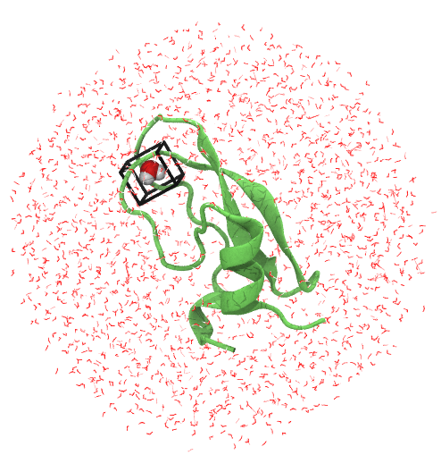
While your visualising the system, have a look at the cysteine bridges. These need to be restrained in ProtoMS which protoms.py will do automatically when preparing proteins. To see that protein_pms.pdb specifies which residues to restrain, open it up and see

REMARK chunk fixresidues 1 5 14 30 38 51 55
REMARK chunk fixbackbone 1 4 6 13 15 29 31 37 39 50 52 54 56

This fixes the cysteine residues, as well as the neighbouring residues. If the above isn't included, the cysteine bonds will break due to a quirk in the backbone sampling of ProtoMS.

Execution

Notice that in the command file run_gcmc.cmd file there is the line

multigcmc 100000 -9.110 -10.110 -11.110 -12.110 -13.110 -14.110 -15.110 -16.110 -17.110 -18.110 -19.110 -20.110 -21.110 -22.110 -23.110 -24.110

An individual simulation will be run at each of these B values with replica exchange moves attempted between neighbours every 100,000 MC moves. These sixteen Adams values mean that sixteen cores will be needed to run these simulations. ProtoMS is designed to run mpi, so to execute, enter

mpirun -np 12 $PROTOMSHOME/protoms3 run_gcmc.cmd

This will take approximately five to six hours to run. The length of time and number of jobs means that it is more convenient to run on a computer cluster than your work-station.

Analysis

Visually inspect your simulations in VMD or your favourite viewer and make sure nothing untoward has happened. Unlike the viewer Pymol, VMD has a problem with simulations that change the total number of molecules. To view a movie of the simulation, a script is provided that modifies the pdb file output by ProtoMS. Pick an middling B value from the folders in out_gcmc and within it, run:

python $PROTOMSHOME/tools/make_gcmc_traj.py -i all.pdb -o mod.pdb -n 1
vmd mod.pdb

and make sure the simulation looks okay. If you chose an appropriate B value you should see a water appearing and disappearing within the binding site.

We can look at the occupancy of the water molecule in each of the simulations. At less negative Adams values, the water has a greater probability to be inserted for the majority of the simulation. In simulations with low Adams values, the water may completely vacate the cavity. Intermediate Adams values will produce a large number of insertions and deletions. Lets have a look at one such intermediate value. For instance, type

python $PROTOMSHOME/tools/calc_series.py -f out_gcmc/b_-19.110/results -s solventson

You may see something like this

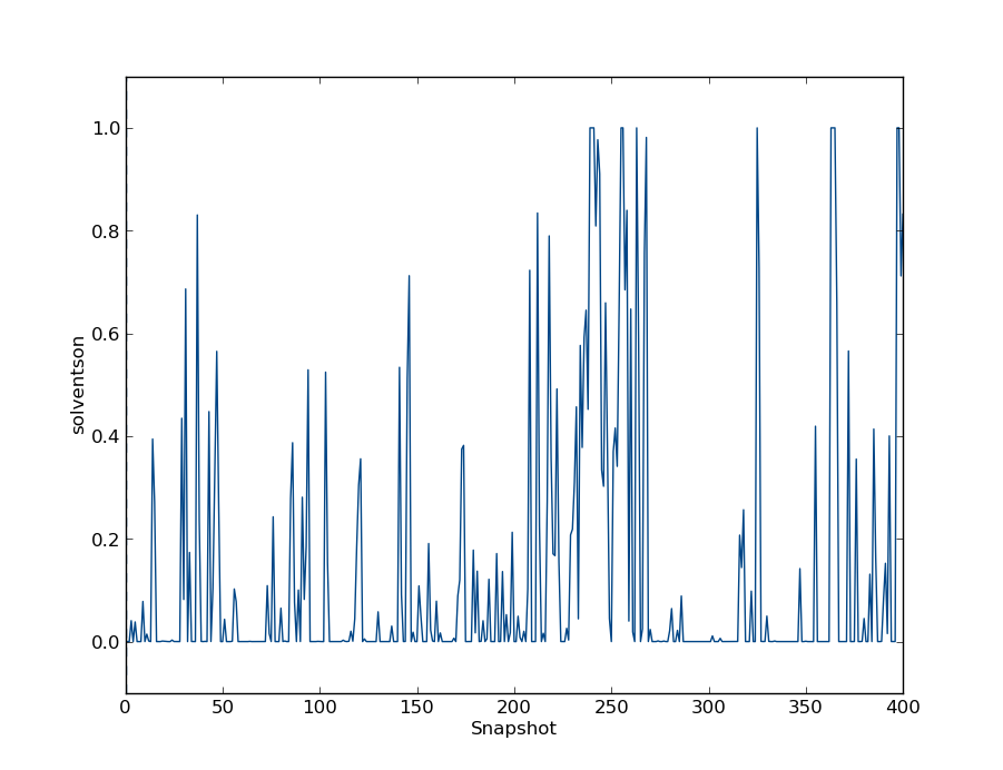
The above shows averages over blocks of the simulation, so non-integer occupancies are expected. Have a look at the corresponding plots for the other simulations.

As demonstrated in G. A. Ross et. al, Journal of the American Chemical Society, 2015, the relationship between the Adams value and the average occupancy of the GCMC region can be used to calculate the free energy to transfer the water molecule from ideal gas to the GCMC region via

‹N› = 1/(1 + exp(βΔF_trans - B)),

where ‹N› is the average number of water molecules, B is the Adams value, ΔF_trans is the free energy to transfer the water molecule from ideal gas, and β is 1/k_BT, with k_B denoting Boltzmann's constant, and T the temperature. This equation - a logistic equation - takes the form of a smooth step function, with the point of inflection given by ΔF_trans. While the transfer free energy can be estimated by eye, the most accurate way to calculate ΔF_trans is to fit the logistic equation to the titration data, as ΔF_trans is the only unknown in the equation. The transfer free energy can be calculated by typing

python $PROTOMSHOME/tools/calc_gcsingle.py -d out_gcmc/b_-* -v 116.5 -p

where the -p flag specifies that titration data and fitted logistic curve will be plotted. The -v flag is the volume of the gcmc region in the simulation in Å³. This was output when make_gcmcbox.py was run, but can also be calculated by the x,y and z dimensions in the gcmc_box.pdb file. The binding free energy of the water molecule calculated by gcmc will be corrected to the standard state, using the term

1/β ln (V/V^o)

where V^o is the standard volume of water in bulk water, 30 Å³. The script calc_gcsingle.py estimates the error in the calculated free energy by performing 1000 bootstrap samples of the titration data and refitting the logistic equation each time. The printed results should look something like:

FREE ENERGY ESTIMATES WITH VOLUME CORRECTION:
  Least squares estimate = -11.05 kcal/mol
  Bootstrap estimate     = -11.04 +/- 0.06 kcal/mol

The first result, Least squares estimate, is simply the least squares fit of the transfer free energy, and has no error associated with it. The second result, Bootstrap estimate is the estimate that has been calculated via bootstrap sampling. The value quoted is the mean transfer free energy from all bootstrap samples, and the error is the standard deviation from those samples. To get the binding free energy of water for the GCMC region, simply take the difference of the transfer free energy and hydration free energy of water. ProtoMS calculates the hydration free energy of water to be about -6.2 kcal/mol, so the binding energy is roughly -11.0 + 6.2 = -4.8 kcal/mol.

Two plots will have been produced when calling calc_gcsingle.py. Like the results, one shows the least squares fit of the logistic function, and the second shows the results of the bootstrap sampling and fitting, and is probably more informative. For the latter, you may see something like

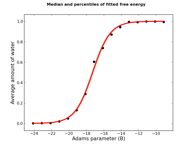
The red line marks the median of the all the bootstrap fits. Typically, orange and grey areas on these plots highlight the regions of 50% and 90% of all the fits respectively. In this figure, as all of the data points are so close to the line all of the bootstrapped fits are very consistent, so only a small region of grey can be seen. To be clear, these errors illustrate the uncertainty of the fit, not the GCMC titration data. The error produced from the bootstrap sampling can be reduced with data more GCMC simulations, particularly at Adams values near the point of inflection.

Exploring more options

Here, we'll consider some points that will help with the set-up and execution of GCMC on a single water molecule.

Setting the Adams values

The Adams parameter affects the probability to accept and insert or deletion move. Lowering the Adams value makes it more likely to empty the GCMC simulation region, while raising the Adams value increases the occupancy of the cavity. It is recommended to include the B_equil value in your simulations, either as a single value, or within a range of simulated B values.

--adams - input the Adam(s) value(s) you want to simulate at.

If only one value is entered, for instance

python $PROTOMSHOME/protoms.py -sc protein_pms.pdb -s gcmc --gcmcwater wat.pdb --gcmcbox gcmc_box.pdb --adams -9.11

the command file run_gcmc.cmd will have the line

potential -9.110

On the other hand, if one were to enter multiple Adams values, for instance

python $PROTOMSHOME/protoms.py -sc protein_pms.pdb -s gcmc --gcmcwater wat.pdb --gcmcbox gcmc_box.pdb --adams -9 -10

one would find this line in run_gcmc.cmd:

multigcmc 100000 -9.000 -10.000

where B_equil is within the range of B values. The difference between these two commands determines whether one needs to run ProtoMS with MPI. For one Adams value, ProtoMS is executed with

$PROTOMSHOME/protoms3 run_gcmc.cmd

With more than one value, ProtoMS is executed with

mpirun -np 16 $PROTOMSHOME/protoms3 run_gcmc.cmd

were 16 would typically be the number of b values in the simulation. When choosing which Adams values to use in ones simulations, note βΔF_trans is the point of half maximum of the logistic curve. Reliable transfer free energy estimates can be achieved with the Adams values around this point.

start by simulating with values between -16 and 0 and analysing the results. You can choose more Adams values to simulate with if you didn't get reliable free energy estimates from the runs you already have.

Running independent repeats

Multiple independant repeats are essential for well resolved free energy estimates. Every GCMC simulation counts as an individual repeat, and one can always run additional simulations at different Adams values. If you're sure of the Adams value(s) from the start and want, say, 3 repeats, typing

python $PROTOMSHOME/protoms.py -sc protein_pms.pdb -s gcmc --gcmcwater wat.pdb --gcmcbox gcmc_box.pdb --adams -9 -10 -11 -r 3

will create 3 command files called run1_bnd.cmd, run2_bnd.cmd, and run3_bnd.cmd, which, when executed, create the output folders out_gcmc1, out_gcmc2, and out_gcmc3. Analysing the results from multiple directories is trivial; all you need to do is enter the directories that contain the ProtoMS results files. For instance, one can type

python $PROTOMSHOME/tools/calc_gcsingle.py -d out_gcmc1/b_-* out_gcmc2/b_-* out_gcmc3/b_-*

to analyse all the simulation data in one go.

Setting the move proportions for GCMC

The default behaviour in protoms.py when assigning move proportions is to dedicate half of all trial moves to grand canonical solute moves. A typical run_gcmc.cmd created by protoms.py for BPTI will contains the lines

chunk equilibrate 5000000 solvent=0 protein=0 solute=0 insertion=333 deletion=333 gcsolute=333
chunk equilibrate 5000000 solvent=440 protein=60 solute=0 insertion=167 deletion=167 gcsolute=167
chunk simulate 40000000 solvent=440 protein=60 solute=0 insertion=167 deletion=167 gcsolute=167

Note how the numbers to the right of each "=" sign roughly add up to 1000.The terms insertion, deletion, and gcsolute are specific to GCMC. Let's look at the last two chunks. As 167+167+167≈500, the proportion of moves dedicated to GCMC is 500/1000=1/2. This default behaviour was designed for cases when the GCMC region would contain tens of water molecules, and not just one water molecule as we have with BPTI. By trailing too many moves on the single water molecule in the BPTI case, we run the risk of undersampling the rest of the system with respect to the water molecule. While that isn't the case with BPTI, it may be for other systems, so it's worth experimenting with different move proportions. Altering the last two chunks to read

chunk equilibrate 5000000 solvent=440 protein=60 solute=0 insertion=50 deletion=50 gcsolute=50
chunk simulate 40000000 solvent=440 protein=60 solute=0 insertion=50 deletion=50 gcsolute=50

means that one fifth of all moves will be dedicated to sampling the grand canonical water molecule. The free energy calculated from such simulations is not significantly different to what we calculated before for BPTI, which lends confidence in our estimate.

Files created by the setup script

Simulation specific files

Running make_gcmcbox.py and protoms.py created the following files:

gcmc_box.pdb = the box that marks out the volume where GCMC will be carried out; created by mark_gcmcbox.py
gcmc_wat.pdb = a water molecule that GCMC moves will be performed on
water.pdb = the droplet of solvent water that surrounds the protein
run_gcmc.cmd = the command file that tells ProtoMS what to simulate and how

If there were any molecules from water.pdb that were within the GCMC box, they would be removed and the file water_clr.pdb will be created as well.

Setting up the simulation with individual tools

Here, we'll go through through the set-up of the ProtoMS files step by step, we'll also do without the help of the automatisation in protoms.py. Doing so will grant us some extra flexiblity.

Setting up the GCMC box

Before running GCMC, you have to be very clear what region you want to allow GCMC moves. In the example BPTI example at the top of the page, we used make_gcmcbox.py to delineate the volume around the structure wat.pdb. If you don't have such a structure to draw a box around, you can also specify the size and centre of the box instead. For instance,

python $PROTOMSHOME/tools/make_gcmcbox.py -b 32.67 4.32 10.34 -p 2 -o gcmc_box.pdb

will create gcmc_box.pdb centered around x=32.67, y=4.32 and x=10.34, with 2 Angstroms either side of the centre such that the box has a volume 4×4×4 Angstroms cubed. Alternatively, one can create the same box by specifying

python $PROTOMSHOME/tools/make_gcmcbox.py -b 32.67 4.32 10.34 4 4 4 -o gcmc_box.pdb

Here, we've explicitly stated the size of the box in each direction, meaning we could create a cuboid by giving different box lengths in each direction, as opposed to the cube with the -p flag.

Solvating the system

To solvate the protein with a sphere of water, up to a radius of 26 Angstroms, one can enter the following:

python $PROTOMSHOME/tools/solvate.py -pr protein_pms.pdb -g droplet -r 26 -b $PROTOMSHOME/data/wbox_tip4p.pdb -o water.pdb

This makes water.pdb. We need to specify the water molecules that we'll be sampling with GCMC. We'll use solvate.py again to fill the volume specified by gcmc_box.pdb.

python $PROTOMSHOME/tools/solvate.py -pr gcmc_box.pdb -g flood -b $PROTOMSHOME/data/wbox_tip4p.pdb -o gcmc_wat.pdb

with output gcmc_wat.pdb. When running Monte Carlo, ProtoMS will not allow any bulk water molecules (specified in water.pdb) to enter or leave the dimentions specified in gcmc_box.pdb. So that we don't block the movement of the grand canonical water molcules (specified in gcmc_wat.pdb), we need to remove any block water molecules that are with the box:

python $PROTOMSHOME/tools/clear_gcmcbox.py -b gcmc_box.pdb -s water.pdb -o water_clr.pdb

In the BPTI test case, no water molcules in water.pdb are within the GCMC region, so no waters are cleared and, in this case, we don't need the created file water_clr.pdb.

Making the ProtoMS input file

The make the input file for the Monte Carlo simulation, we reference the files created thus far

python $PROTOMSHOME/tools/generate_input.py -s gcmc -p protein_pms.pdb -pw water.pdb --gcmcwater gcmc_wat.pdb --gcmcbox gcmc_box.pdb --adamsrange -9.110 -24.110 -o run

creating run_gcmc.cmd.